Naive diffuse path tracing #

Overview #

In the following sections, I want to describe how naive diffuse path tracing works. The goal of this chapter is to give you an understanding of how the following scene can be rendered:

Cornell Box rendered with naive diffuse path tracing

The scene shows the Cornell Box. Furthermore, it shows some nice effects such as soft shadows and light bleeding (the tall block receives “red light” from the red wall - the short block gets “green light” from the green wall).

To understand this article you should be able to implement at least a simple raycaster that is capable of rendering the albedo color for the Cornell Box scene, like this:

Cornell Box albedo

Once you have this starting point you can dive into this article.

In the following, we will cover different topics: The rendering equation, Lambert’s cosine law, ideal diffuse surfaces & reflection, Monte Carlo integration, and finally the basics of path tracing.

The rendering equation #

This is the rendering equation (to be more exact one form of its representation):

\[L_o(x,\omega_o)= L_e(x,\omega_o) + \int_{\Omega^{+}} f_r(x, \omega_i, \omega_o) L_i(x,\omega_i) (\omega_i \cdot n) d\omega_i\]

The following figure shows some of the variables involved in this equation:

The rendering equation

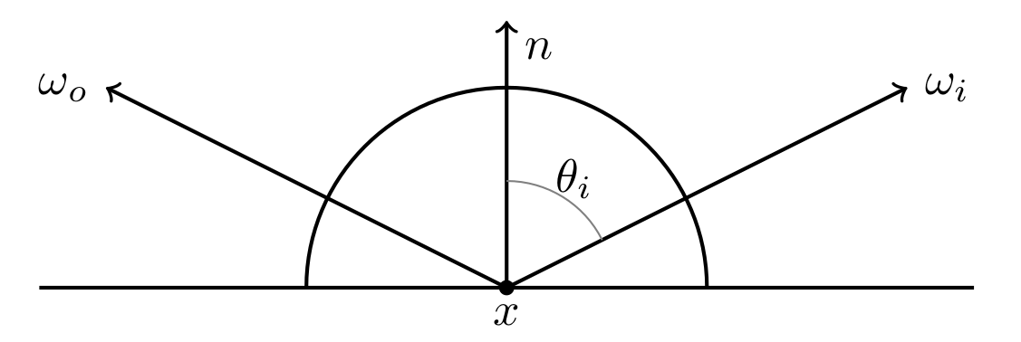
The rendering equation describes how much light \(L_o\) arrives from a specific location \(x\) coming from a specific direction \(\omega_o\) . \(L_o\) is the sum of the light that is emitted at the location \(x\) and forwarded into the direction of \(\omega_o\) and the incoming light \(\omega_i\) towards \(x\) that is reflected towards \(\omega_o\) . \(f_r(x,\omega_i,\omega_o)\) describes which partition of the incoming light is reflected toward the outgoing reflected light direction \(\omega_o\) . The term \(\omega_i \cdot n\) is used to take Lambert’s cosine law into account.

There are some conventions:

The index \(i\) is used to denote incoming light
The index \(o\) is used to denote outgoing light
The index \(e\) is used to denote emitted light
\(x\) , \(\omega_o\) , \(\omega_i\) , \(n\) are vectors
\(\omega_i\) points always into the negative direction of the incoming light
\(\omega_i\) , \(n\) are assumed to be normalized
\(n\) is a normal vector
\(\Omega^{+}\) describes the positive hemisphere around \(n\)
sometimes \(\cos{\theta_i}\) is used instead of \(\omega_i \cdot n\) . \(\theta_i\) is the angle between \(n\) and \(\omega_i\)
\(f_r\) is a bidirectional reflectance distribution function (BRDF) that describes how much of the light with the incoming direction \(-\omega_i\) is reflected towards \(\omega_o\)

Let me repeat this (repetition helps to learn): The rendering equation says all light that arrives from some location at the eye of an observer is the sum of the light that is directly emitted from that certain location and the incoming light at that location that is reflected towards the observer.

The rendering equation in the shown form can not model all effects of the interaction of light with matter, but serves as an easy formulation to describe global illumination effects that as shadows or color bleeding. Light can be considered at different wavelengths \(\lambda\) and therefore the rendering equation could also be extended with it (i.e. \(L(x,\omega_o,\lambda)\) ). Nevertheless, spectral rendering, which would consider different wavelengths \(\lambda\) , is outside of the scope of this article.

Lambert’s cosine law #

Imagine a light bundle that hits one square meter orthogonal. Now let us rotate this light bundle a bit. What can we observe?

Lambert’s cosine law

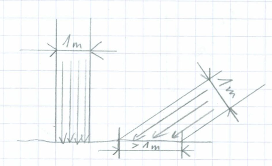
The rotated light bundle is distributed now to more than one square meter. So to say, the same energy is distributed to more area.

Assuming that \(\omega_i\) and \(n\) are normalized vectors the scalar product of these two vectors accounts for this effect. If both vectors are identical (meaning the light bundle hits the floor orthogonal) the scalar product is \(1\) . If both vectors are parallel (no light hits the floor) the scalar product is \(0\) . If both vectors point in opposite directions the scalar product is \(-1\) . The case of a negative scalar product has not to be considered here, since we only consider here the positive hemisphere.

Assuming you have a solar panel. The more the normal of the surface of the normal and the incoming light direction fits so more solar power you get.

To account for this in the rendering equation we have the term

\[\cos{\theta_i} = \omega_i \cdot n\]

The physical principle behind this is called Lambert’s cosine law.

Ideal diffuse surfaces & reflection #

Hemispherical-directional reflectance #

The hemispherical-directional reflectance (albedo \(\rho\) ) is defined as

\[\rho = \int_{\Omega^{+}} f_r(x, \omega_i, \omega_o) (\omega_i \cdot n) d\omega_i\]

When taking a closer look at the hemispherical-directional reflectance equation it is very similar to the rendering equation. The only thing that is missing is the “light term” \(L_i\) . Actually, it is not missing but it is set to a constant value of \(1\) . This means \(\rho\) will tell us the “color” of an object that is uniformly lit and is this way somehow independent of a concret lighting environment.

To be more formal \(\rho\) describes the amount of light that is reflected along a given direction \(\omega_o\) for incoming light in any direction in the hemisphere around the surface normal.

Diffuse reflection (Lambertian BRDF) #

A simple BRDF is the Lambertian BRDF. A lambertian BDRF is a BRDF that is constant for every incoming direction \(\omega_i\) , outgoing direction \(\omega_o\) , and sample position \(x\) , i.e.

\[f_r(x,\omega_i,\omega_o) = f_\text{lambert} = const = \frac{\rho}{\pi}\]

The lambertian BRDF is invariant to the incoming directions of light which means it reflects every incoming light ray in the same uniform way. Every incoming light ray is reflected equally in all outgoing directions. A surface that has this property is also called a diffuse surface.

Since \(f_\text{lambert} = const\) , we can write:

\[\rho = f_{lambert} \int_{\Omega^{+}}(\omega_i \cdot n) d\omega_i\] \[f_{lambert} = \frac{\rho}{\int_{\Omega^{+}}(\omega_i \cdot n) d\omega_i}\]

It turns out that for the lambertian BRDF the following holds:

\[f_{lambert} = \frac{\rho}{\pi}\]

The derivation of this can be seen here.

Monte Carlo Integration #

In the case, our scene consists only of diffuse materials (described by a Lambertian BRDF) the rendering equation can be simplified to:

\[L_o(x,\omega_o) = L_e(x,\omega_o) + \frac{\rho}{\pi} \int_{\Omega^{+}} L_i(x,\omega_i) (\omega_i \cdot n) d\omega_i\]

This integral can be solved using Monte Carlo integration:

\[\int_a^b f(x) dx \approx \frac{1}{N} \sum_{i=0}^{N-1}{\frac{f(x_i)}{p(x_i)}}\]

Monte Carlo integration works by generating random numbers \(x_i\) in the integration domain \([a,b]\) with an arbitrary density \(p\) . The only condition here is that \(p\) needs to fulfill the properties of a probability density function (PDF). More details on why this works can be found here.

Applied to our integral we can write:

\[\int_{\Omega^{+}} L_i(x,\omega_i) (\omega_i \cdot n) d\omega_i \approx \frac{1}{N} \sum_{i=0}^{N-1}{\frac{L_i(x,\omega_i) (\omega_i \cdot n)}{p(\omega_i)}}\]

This means:

\[L_o(x,\omega_o) \approx L_e(x,\omega_o) + \frac{\rho}{\pi} \frac{1}{N} \sum_{i=0}^{N-1}{\frac{L_i(x,\omega_i) (\omega_i \cdot n)}{p(\omega_i)}}\] \[L_o(x,\omega_o) \approx \frac{1}{N} \sum_{i=0}^{N-1}L_e(x,\omega_o)+\frac{\rho}{\pi}{\frac{L_i(x,\omega_i) (\omega_i \cdot n)}{p(\omega_i)}}\]

\(p(\omega_i)\) can be chosen arbitrarily, e.g.: \(p(\omega_i) = \frac{\cos{\theta}}{\pi} = \frac{\omega_i \cdot n}{\pi}\)

This simplifies the equation to

\[L_o(x,\omega_o) \approx \frac{1}{N} \sum_{i=0}^{N-1}L_e(x,\omega_o)+\frac{\rho}{\pi}{\frac{L_i(x,\omega_i) (\omega_i \cdot n)}{ \frac{\omega_i \cdot n}{\pi} }}\] \[L_o(x,\omega_o) \approx \frac{1}{N} \sum_{i=0}^{N-1}{L_e(x,\omega_o) + \rho L_i(x,\omega_i) }\]

When drawing samples for \(\omega_i\) it must be ensured that the samples are distributed according \(p(\omega_i) = \frac{\cos{\theta}}{\pi}\) , i.e. they must be cosine distributed.

Path Tracing #

To render our scene we shot rays from the virtual eye point into our scene. When a ray hits an object, we need to trace \(N\) number of rays over the hemisphere of all incoming light directions \(L_i\) .

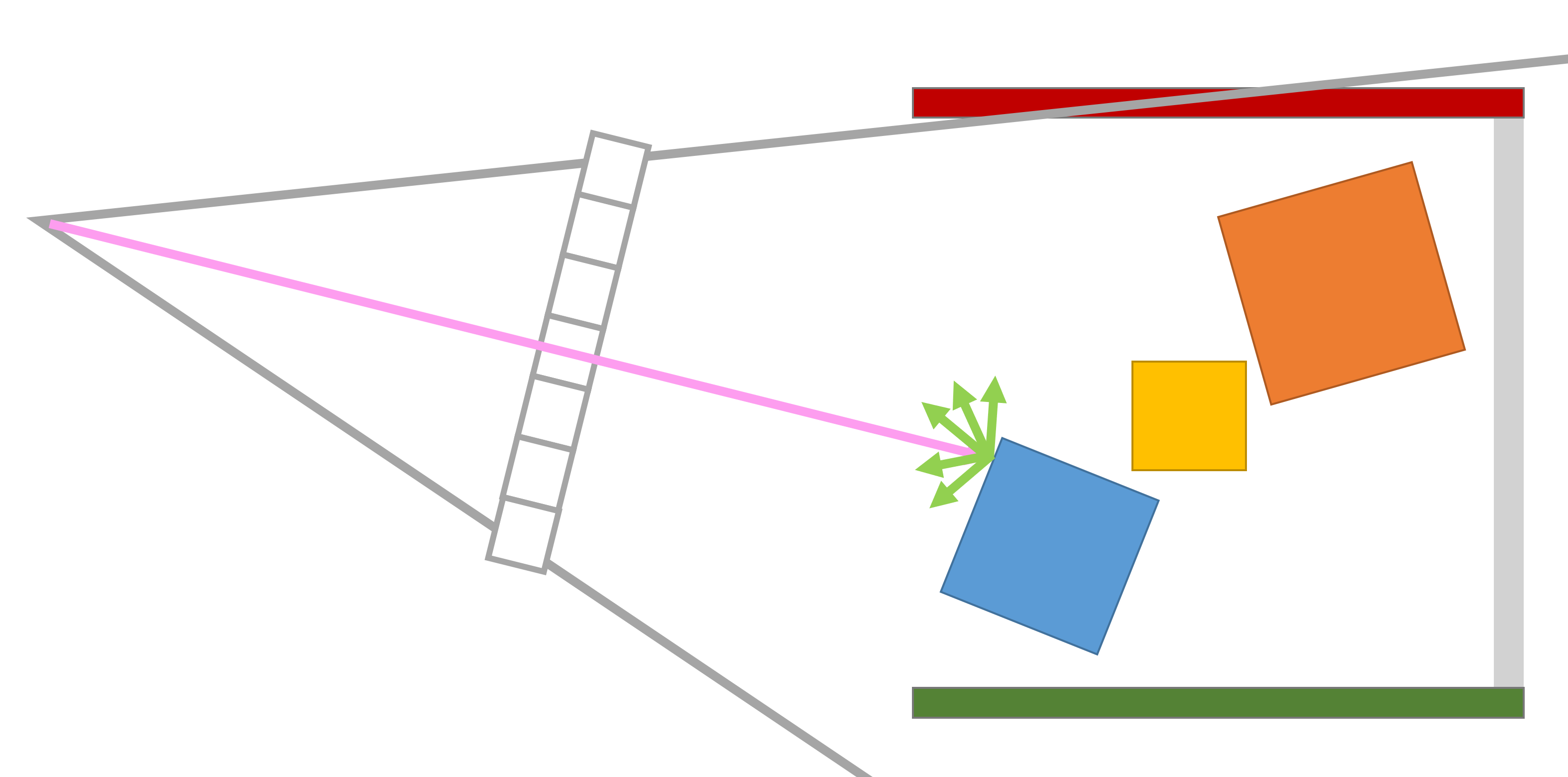Cornell Box rendered with ray tracing For each follow-up ray, we have to sample again the whole hemisphere. This can be done, but the rays we have to follow will grow exponentially.

The idea of path tracing is to set \(N\) to \(1\) to follow only one light path:

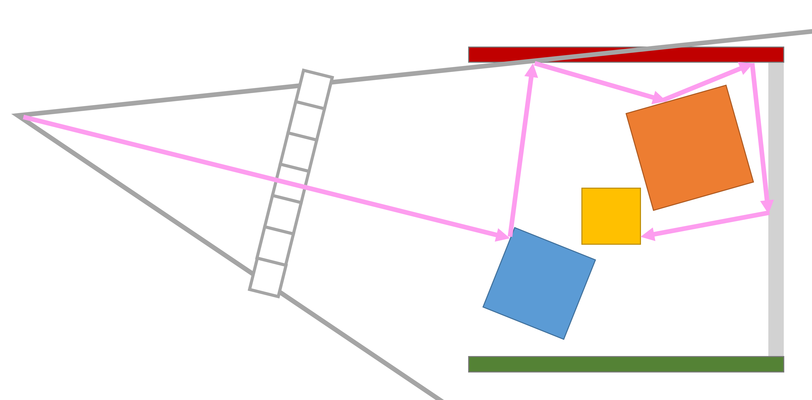
Cornell Box rendered with ray tracing

By repeating this path-tracing process many times for each pixel (samples per pixel) an averaging the results we get a converging image.

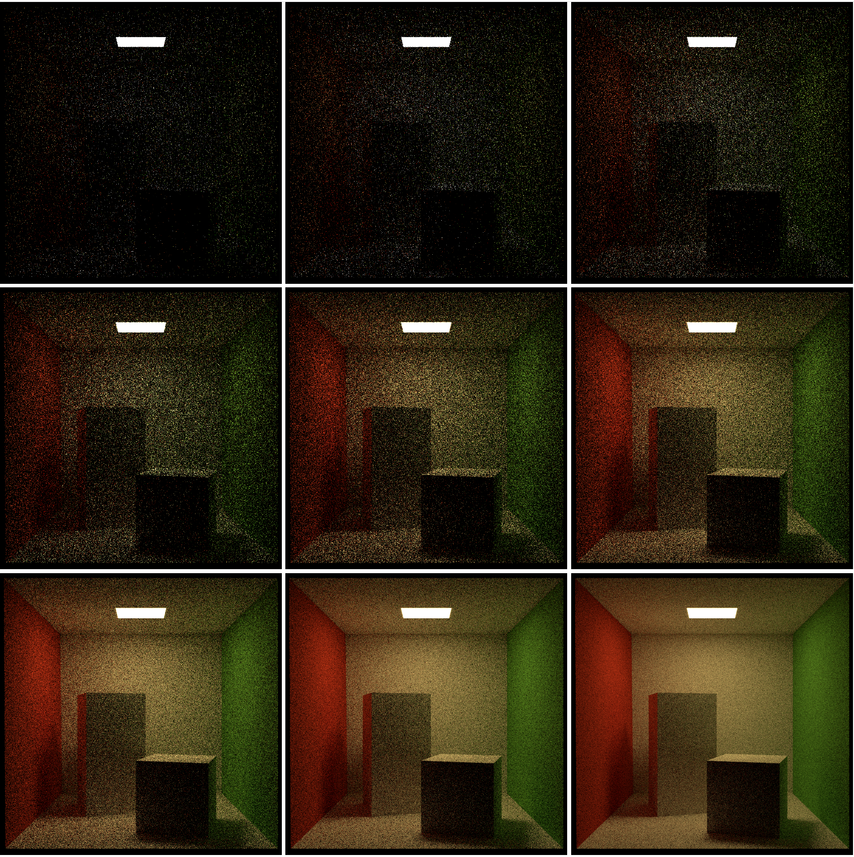
Cornell Box rendered with different sample per pixel counts

Since naive diffuse path tracing as described here is only following a ray path. If the path hits something, we sample a cosine-weighted hemisphere direction and go on. By doing this a ray send from the camera center to the “middle” of the Cornell Box will only hit with a probability of about \(5\%\) the light source and also only those \(5\%\) will contribute to the final image. Therefore, this technique is very slow and converges slowly.

Implementation #

Coordinate system for BRDFs #

BRDFs use normally coordinates where the z-axis is aligned with the surface normal \(n\) (e.g. see here). Since usually a world space coordinate system is used where the y-axis points upwards, it must be ensured that a proper basis transform is done, before a BRDF is evaluated.

A trace function for naive diffuse path tracing #

A function for naive diffuse path tracing can look like this:

virtual Color trace(
      const Scene *scene,
      Sampler* sampler,
      Ray &ray,
      const int depth) const {
        MediumEvent me;
        if (scene->intersect(ray, me) && depth < max_depth_) {
            Color emitted_radiance{0, 0, 0};
            if(me.shape->is_emitter()) {
                emitted_radiance += me.shape->emitter()->evaluate();
            }

            auto sample = sampler->next_2d();

            const Scalar EPSILON =  Scalar{0.0001};
            Vector wi = cos_weighted_random_hemisphere_direction(me.sh_frame, sample);
            Ray rn(me.p, wi, EPSILON, std::numeric_limits<Scalar>::infinity());
            Vector wo = -ray.direction;

            Color color{0.f};
            if(me.shape->bsdf()) {
                color = me.shape->bsdf()->evaluate(wo, wi) * pif; // we need to undo the \pi term
            }

            return emitted_radiance + color * trace(scene, sampler, rn, depth + 1);
        }
        else {
            return Color{0, 0, 0};
        }
    }