Image sampling and reconstruction #

Pixel positions #

Integer coordinates can be used to address different positions on a discrete pixel image grid. Usually, the top left pixel has the coorinates \((0,0)\) and the bottom right one \((width-1,height-1)\) . This is space is called the raster space.

When sampling an image plane we use floating-point coordinates. One important question is how to convert from discrete coordinates to continuous ones and vice versa. Paul Heckbert has written a nice article about this (What Are the Coordinates of a Pixel?, Paul S. Heckbert, Graphics gems, August 1990 Pages 246–248). He introduces a rounding and a truncating scheme as shown in the next image.

In this article, I assume a truncating scheme is used, which means pixel \((4.9,1.0)\) would address the discrete pixel \((4,1)\) . In a rounding scheme, the pixel \((5,1)\) would be addressed by the aforementioned floating-point coordinates.

The truncating scheme offers the advantage that we need not to deal with negative coordinates nor doing rounding to convert between discrete and continuous coordinates.

Aliasing #

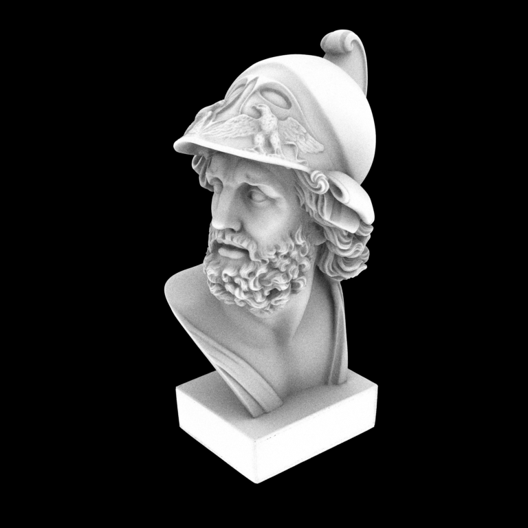
The absence of proper image sampling and reconstruction can lead to several problems, such as aliasing as depicted in the following image (rendering of Ajax model).

The Ajax model was sampled using the pixel center for each traced ray, which leads to jagged edges between the background and the Ajax model. \(256\) samples per pixel were used to render this image. For every sample, the pixel center \((x+0.5,y+0.5)\) was sampled and the determined ambient occlusion was accumulated. The next figure shows an example of the used sampling pattern.

Even when changing the sample pattern in a way that random positions for each sample are chosen within the pixel boundaries the jagged edges remain.

What really does the trick here is image filtering. There are several prominent image filtering techniques:

• B-Spline Cubic Filter
• Box Filter
• Catmull-Rom Filter/Catmull-Rom Cubic Filter
• Gaussian Filter
• Mitchell Filter/Mitchell-Netravali Cubic Filter
• Tent Filter/Triangle Filter/Hat Filter
• Lanczos Filter/Windowed Sinc Filter

Tent filter #

Let’s have a look at the tent filter:

Tent Filter	1D	2D
Function	\(f_{tent1d}(x)=1-\|x\|\)	\(f_{tent2d}(x,y)=(1-\|x\|)\cdot(1-\|y\|)\)
Impulse response
Contour plot

Assuming you want to apply some radius \(r\) in the 1D case or \((r_x,r_y)\) in the 2D case to the tent filter, the filter functions are computed by:

Of course, the support of the tent filter has to be restricted to some interval. For \(x\) to \(|x| < 1\) and for y to \(|y| < 1\) .

The plot of a tent filter of radius \(100 \times 100\) looks like this (very a cold hot color ramp was applied):

Filtering #

Every sample with continuous pixel coordinates \((x_i,y_i)\) within the filter radius contributes to a final pixel value:

Implementation idea:

class Film {
public:
    Film(...) {
        // ...
        filterWeightSums_ = new float[width*height];
        radianceSum_ = new Color3f[width*height];

        for (int i = 0; i < width*height; ++i) {
            filterWeightSums_[i] = 0.0f;
            radianceSum_[i] = Color3f{0.f, 0.f, 0.f};
        }
    }
    void addSampleSlow(const Point2f& samplePosition, const Color3f& color) {
        for(int y = 0; y < image_->getHeight(); ++y) {
            for(int x = 0; x < image_->getWidth(); ++x) {
                float filterWeight = filter_->evaluate(Point2f{dx,dy});

                if(filterWeight > 0.f) {
                    filterWeightSums_[x+y*image_->getWidth()] += filterWeight;
                    radianceSum_[x+y*image_->getWidth()] += filterWeight * color;

                    // update pixel
                    float totalWeight = filterWeightSums_[x+y*image_->getWidth()];
                    Color3f totalRadiance = radianceSum_[x+y*image_->getWidth()];
                    image_->setPixel(x,y, (1.f/totalWeight) * totalRadiance);
                }
            }
        }
    }

    // ...

private:
    float* filterWeightSums_ = nullptr;
    Color3f* radianceSum_ = nullptr;
}

The above implementation idea does not work in practice because it is too slow. Nevertheless, it shows a very basic implementation idea of image filtering.

Usually, the filter support is restricted locally. This enables us to compute filtering only for those pixels where sampling will have an effect.

void addSample(const Point2f& samplePosition, const Color3f& color) {
    Bounds2i bounds = computeBounds(samplePosition);

    for(int y = bounds.min_v.y(); y < bounds.max_v.y(); ++y) {
        for(int x = bounds.min_v.x(); x < bounds.max_v.x(); ++x) {
            float dx = x + .5f - samplePosition.x();
            float dy = y + .5f - samplePosition.y();

            float filterWeight = filter_->evaluate(Point2f{dx,dy});

            if(filterWeight > 0.f) {
                filterWeightSums_[x+y*image_->getWidth()] += filterWeight;
                radianceSum_[x+y*image_->getWidth()] += filterWeight * color;

                // update pixel
                float totalWeight = filterWeightSums_[x+y*image_->getWidth()];
                Color3f totalRadiance = radianceSum_[x+y*image_->getWidth()];
                image_->setPixel(x,y, (1.f/totalWeight) * totalRadiance);
            }
        }
    }
}

A method name computeBounds was introduced. This is very similar how pbrt does it. computeBounds works by looking at the sample value. For the left boundary is determined by subtracting from the x sample value the filter radius. Afterward, the value \(0.5\) is added and finally, the value is converted to an int.

The following figure shows how to compute the pixel boundaries for relevant pixels.

Bounds2i computeBounds(const Point2f& samplePosition) const {
    Bounds2i bounds;

    bounds.min_v.x() = samplePosition.x() - filter_->getRadius().x() + 0.5f;
    bounds.min_v.y() = samplePosition.y() - filter_->getRadius().y() + 0.5f;

    bounds.max_v.x() = samplePosition.x() + filter_->getRadius().x() - 0.5f;
    bounds.max_v.y() = samplePosition.y() + filter_->getRadius().y() - 0.5f;

    bounds.min_v.x() = std::max(bounds.min_v.x(), 0);
    bounds.min_v.y() = std::max(bounds.min_v.y(), 0);

    bounds.max_v.x() = std::min(bounds.max_v.x()+1, image_->getWidth());
    bounds.max_v.y() = std::min(bounds.max_v.y()+1, image_->getHeight());

    return bounds;
}

For the maximum value, we do it similarly. We add the filter radius and subtract \(0.5\) . In the end, we also add \(1\) since the maximal value should be excluded and not included.

To get a better understanding of image filtering Peter Shirly proposes in his book Realistic Ray Tracing (2nd edition, page 51) the following test function:

Using a tent filter with 100 samples per pixel where the samples are uniform random distributed the following image is generated:

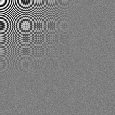
Using a tent filter with 100 samples per pixel where the samples are always centered within the pixel boundaries the following image is generated:

Unit testing #

pbrt-v4 has some unit test implemented for filters.

For several images shown in the blog post, you can come up with a reference image compare test.

For the computeBounds method you can think of simple test cases.

Assuming a filter radius of \(1.0\) you could come up with the following unit test:

//...
Point2f samplePosition = Point2f(101.25f, 102.25f);
Bounds2i b = film->computeBounds(samplePosition);

EXPECT_THAT(b.min_v.x(), 100);
EXPECT_THAT(b.max_v.x(), 102);
EXPECT_THAT(b.min_v.y(), 101);
EXPECT_THAT(b.max_v.y(), 103);

Final words #

The following image shows a rendering of the Ajax model with a tent filter and a radius of \(1\) . Thanks to the tent filter we see fewer jagged edges.

References and Further Reading #

• What Are the Coordinates of a Pixel?, Paul S. Heckbert, Graphics gems, August 1990 Pages 246–248
• Filtering Methods, Page 51, Peter Shirley, Realistic Ray Tracing, 2nd editon
• Antialiasing: To Splat Or Not
• Filter Importance Sampling
• pbrt-v4/src/pbrt/filters_test.cpp
• https://computergraphics.stackexchange.com/questions/3868/why-use-a-tent-filter-in-path-tracing