Chi-squared test applied to sampling #

Some words on notation #

A random variable \(X\) has a probability density function (PDF) \(p\) and a probability distribution function (cumulative distribution function or CDF) \(P\) . \(\xi\) refers to a canonical uniform random variable (uniform distributed variable in the domain [0,1)). \(\omega\) denotes a normalized vector on the unit sphere.

Random number generators #

There are many ways to implement random number generators (RNGs). One of the most basic ones is a linear congruential generator. Of course, there are more advanced ones. One that fits good for ray tracing purposes is PCG. Here is a nice video that gives you an introduction to this kind of random number generator. If you watch the video you will learn that there is a famous test suite for random number generators called TESTU01. It contains different test suites: Small Crush and Big Crush. Surprisingly, most random number generators fail those test suites. If you want to create our own \(\pi\) based random number generator you can use the Nilakantha Series:

A nice library for representing rational numbers to compute approximation of the above series can be found here.

Another interesting question is how one can choose a seed without depending on any machine-related things (such as current time/data, memory addresses, CPU info, etc.). One approach is to provide along with your program a seed.txt that contains a starting seed. Every time the program is started the seed value in the seed.txt gets updated using an RNG. This way every time the program is started gets a new seed value that is independent of any machine’s specifics.

Sampling according to a PDF #

A typical sample problem is that we are given some probability density function (PDF) and we need to generate samples according to this PDF.

Example: The probability density function \(p(x,y)\) is defined by:

How do we generate samples that are distributed according to this PDF? Usually, we assume that we have already solved the problem of uniform distribution of samples in the domain \([0,1(\) , i.e. we have some random number generator that generates uniform random numbers in this domain. How can we use this uniform number generator to generate samples that are distributed to an arbitrary PDF? Since \(p(x,y)\) is composed of two independent 1D distributions, we can solve the problem by considering only \(p_1\) . First we compute the probability distribution function \(P(x)\) (a.k.a cumulative distribution function or cdf) of \(p_1\) .

Now we derive the inverse cdf \(P^{-1}_1\) :

Now we can use \(P^{-1}_1\) to map a uniform random variable \(\xi\) to the \(P(x)\) distribution.

Sample histogram	Integrated density

The Chi-squared test #

The \({\chi}^2\) test can be used to determine if an observed sample distribution matches an expected sample distribution.

For instance, given a sample generator that should generate uniform distributed 2D samples ( \(s_n\) ) within the domain \([0,1) \times x[0,1)\) the \({\chi}^2\) test can be used to check if the generated samples are really uniform distributed. As a null hypothesis, we can formulate that the sample generator generates uniform distributed samples.

The sample generator can be tested by computing the difference between the expected sample frequency ( \(s_e\) ) and the observed sample frequency ( \(s_o\) ) according to (assuming \(s_e \ge 5\) ):

Given a significance level (e.g. 5%) that determines to which degree we allow deviations to the acceptance of our null hypothesis and the given degree of freedom we can determine which value of \({\chi}^2\) is acceptable for us and which not.

To test a continuous 2D sampler you usually divide the domain into a 2D grid (bins). For instance, the domain could be divided in \(51 \times 51\) bins. The degree of freedom is then computed by \(51 \cdot 51-1\) , since the “last” bin is not a real option if all other bins do not fit. Now you count how often a sample lands in a specific bin. At the same time, you know what should be the expected frequency of samples landing in a specific bin. Given those numbers you compute \({\chi}^2\) and given the significance level and degree of freedom, you determine if the null hypothesis is accepted or rejected.

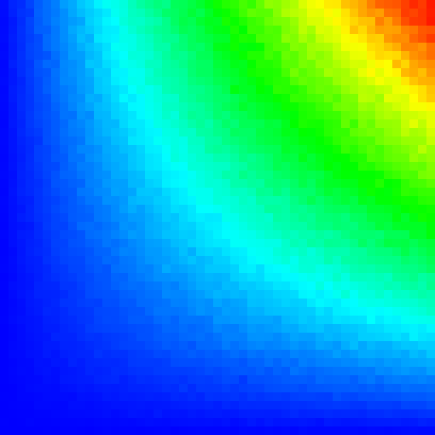
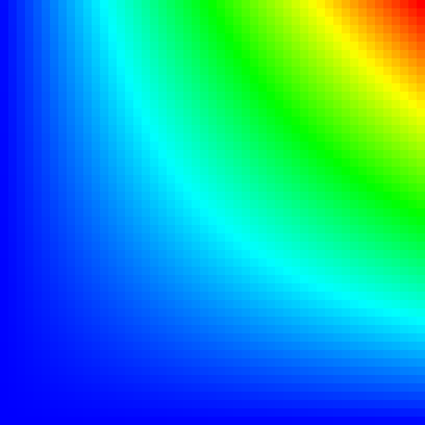
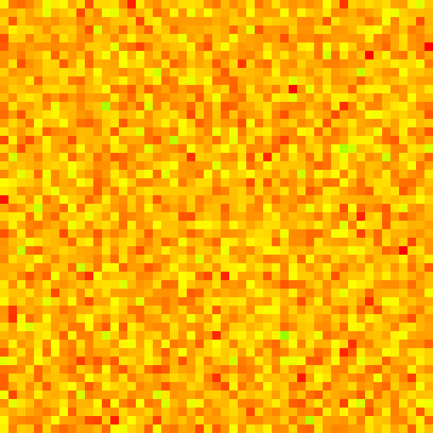
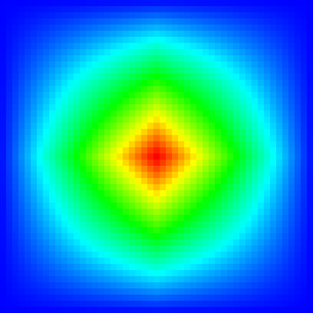
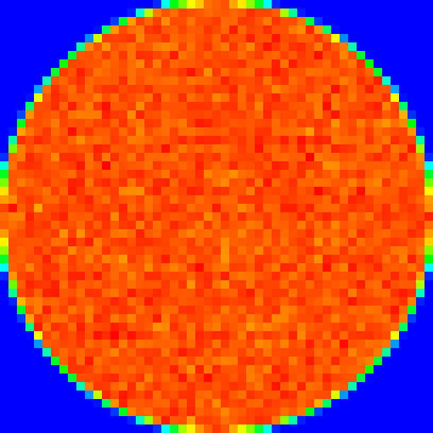
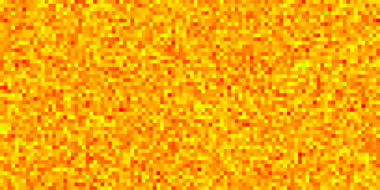
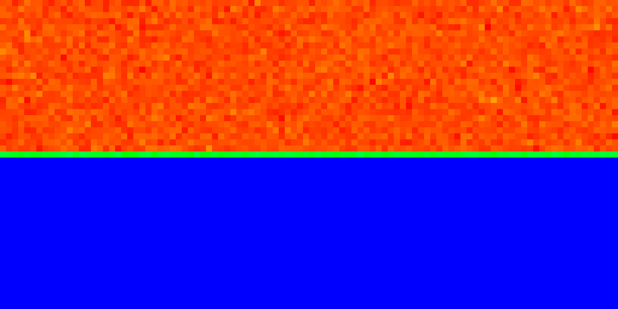
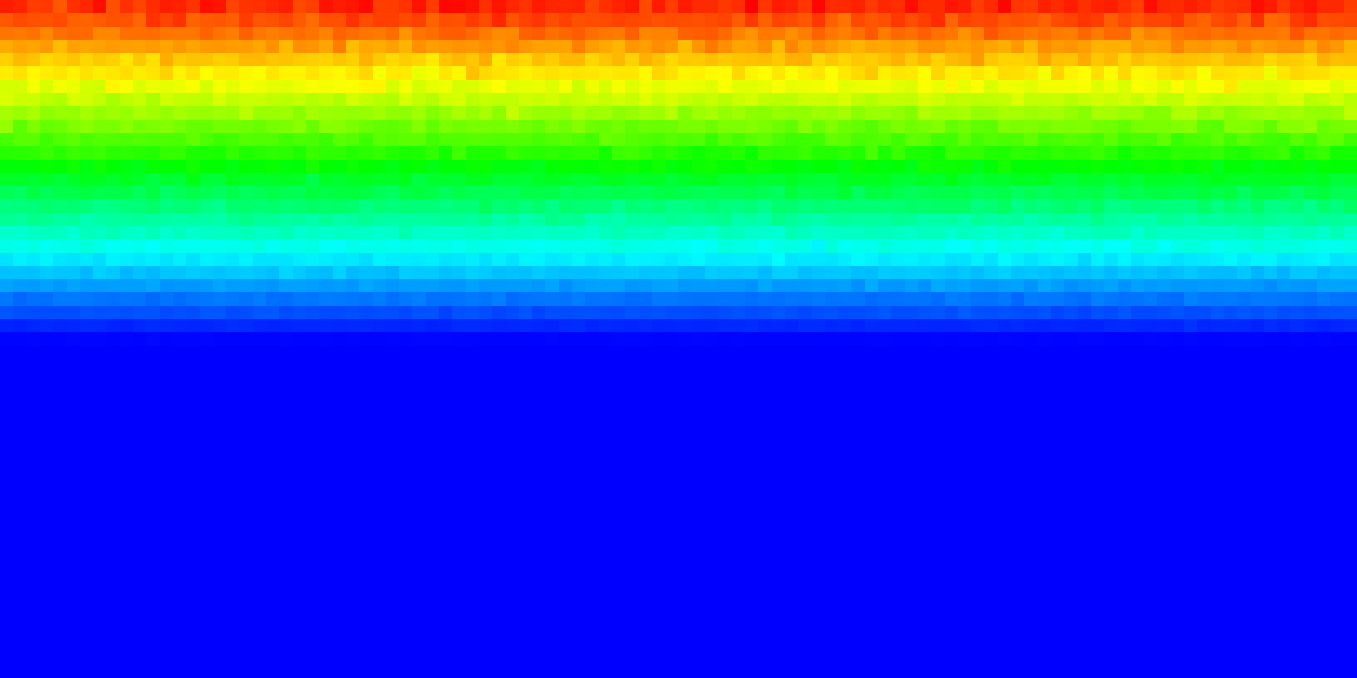
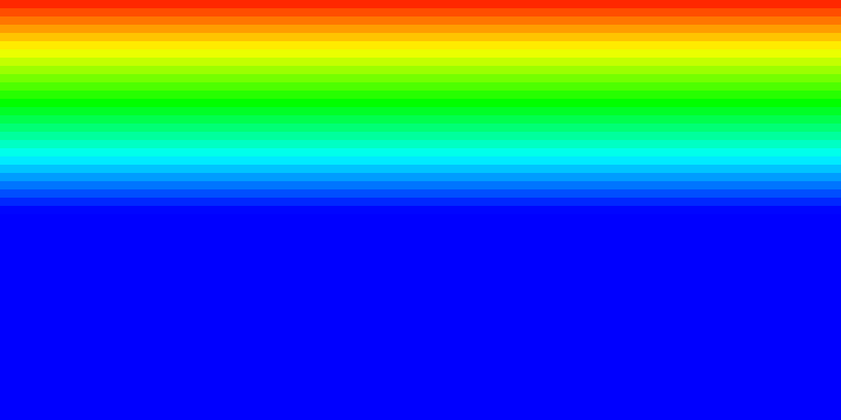
In the following sections, you can see sample histograms and integrated density functions of different distributions. The sample values are summed up using the \({\chi}^2\) test. Visually this means that if the sample histogram and the integrated density (so to say the ground truth) look very similar the sampler seems to work correctly.

Uniform square sampling #

Sample histogram	Integrated density

Tent distribution #

Uniformly distributed 2D points \((x, y) \in [0, 1) \times [0, 1)\) can be converted to a 2D “tent” distribution.

The probability density function (pdf) of the 2D “tent” function is defined by:

Sample histogram	Integrated density

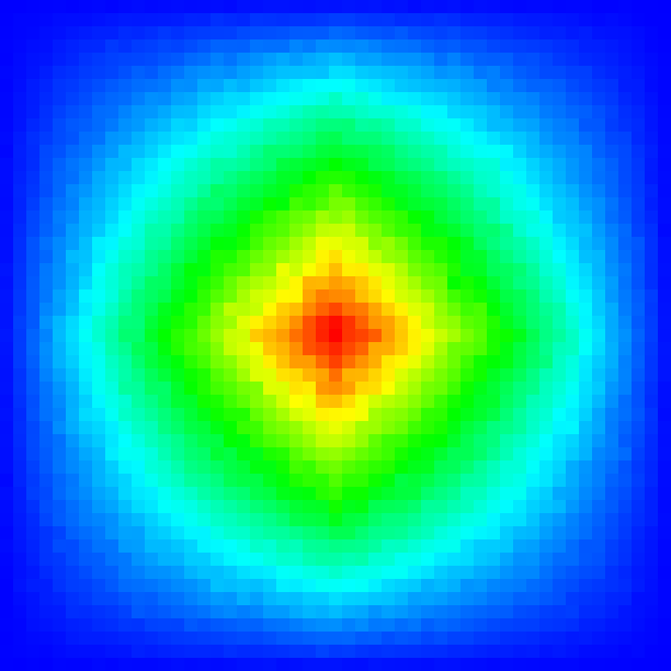Uniform disk sampling #

Sample histogram	Integrated density

Uniform sphere sampling #

Sample histogram	Integrated density

Spherical coordinates (polar coordinates) can be described using a tuple \((r,\theta,\phi)\) that relates to the radial distance (radius) \(r\) , polar angle \(\theta \in [0,\pi)\) , and the azimuthal angle \(\phi ∈[0,2\pi]\) .

Polar coordinates can be converted to cartesian coordinates using the following formulas:

Uniform hemisphere sampling #

Sample histogram	Integrated density

Uniform cosine distributed hemisphere sampling #

Sample histogram	Integrated density

Further reading and references #

• pcg-cpp
• hypothesis.h: A collection of quantiles and utility functions for running Z, Chi^2, and Student’s T hypothesis tests
• Global Illumination Compendium
• Generating uniformly distributed numbers on a sphere
• Chi²-Test: Anpassungstest, Homogenitätstest und Unabhängigkeitstest (German langauge)
• Ideen hinter z-Test, t-Test, chi²-Test, ANOVA; Auswertung in Python (German language)