An interface for a BSDF class #

The goal of path tracing is to solve the rendering equation:

Using the generalized Monte Carlo estimator we can write:

The idea of path tracing is to set \(N\) to \(1\) to follow only one light path:

If we want to formulate this as code, we will come up with something like this:

Li(...) {
    ...
    return = L_e + brdf(...) * Li(...) * cos(theta) / pdf(w_i)
}

In the next section, we will have a more detailed look at how this pseudocode can be extended to get it working with diffuse surfaces.

A Diffuse BSDF class #

A more elaborate pseudocode for a diffuse surface can look like this (taken from here with minor modifications):

Li(Scene scene, Ray ray, int depth) {
    Color emitted = 0;

    if (!findIntersection(scene, ray)) return 0;

    Intersection its = getIntersection(scene, ray);

    // Take care of emittance
    if (isLightSource(its)) emitted = getRadiance(its);

    if(depth >= maxDepth) return emitted;

    // BRDF should decide on the next ray
    // (It has to, e.g. for specular reflections)
    BRDF brdf = getBRDF(its);
    Ray wi = BRDFsample(brdf, -ray);
    float pdf = BRDFpdf(brdf, wi);
    Color brdfValue = BRDFevaluate(brdf, -ray, wo);

    // Call recursively for indirect lighting
    Color indirect = Li(scene, wi, depth + 1);
    return emitted + brdfValue * indirect * cosTheta(wi) / pdf;
}

The idea of the code is to have a BSDF class that provides the methods sample, pdf, and evaluate. Let’s have a closer look at this. We will try now to derive a BSDF interface from this that can at least handle diffuse BRDFs. We start with the pdf member function and add the other functions later. The pdf member function returns the probability that a given direction wi is sampled:

class BSDF {
public:
    [[nodiscard]] virtual float pdf(const Vector3f& wi) const = 0;
};

The pdf member function function expects that wi is a normalized vector on the unit sphere. Furthermore, wi is expected to be given in the reflectance coordinate system. Actually, all vectors handed into the BSDF interface or returned from it use as a basis coordinate system the reflection coordinate system:

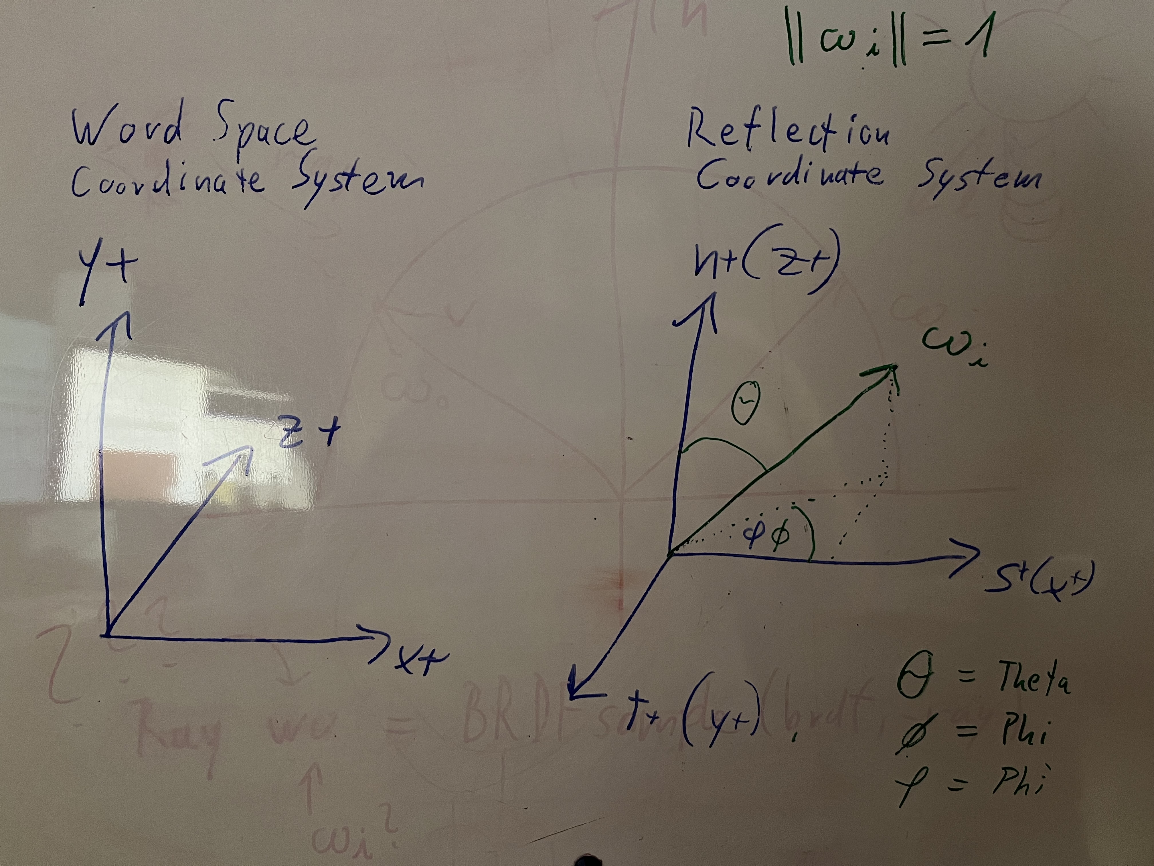
Please note that the reflection coordinate system can be different from the world space coordinate system you are using. I will always make use of the left-handed world space coordinate shown in the image.

When first considering what is prober pdf function you might think for a diffuse BSDF the pdf member function must return a constant value since the probability that an incoming light right ray is reflected in some direction is the same for all directions. This is correct, but we have the freedom to choose any PDF we want. The question is not how a perfect diffuse reflection is distributed, but what is the best strategy to sample it efficiently. Something that is missing in our BSDF class is a sample member function. The sample member function picks a random direction wi for us and the pdf method is expected to reflect the probability density function of those \(\omega_i\) samples. And this does not mean that our samples are uniformly distributed. We could make it that way, but we will go for another distribution (cosine-weighted hemisphere sampling).

Now let us extend the BSDF class with a sample method. The sample function member takes a 2D sample point as input and returns a random sample direction \(\omega_i\) :

class BSDF {
public:
    [[nodiscard]] virtual Vector3f sample(const Point2f& sample_point) const = 0;
    [[nodiscard]] virtual float pdf(const Vector3f& wi) const = 0;
};

If we are handing in only a sampling point to the sample method the BSDF is independent of the normal vector \(n\) at the intersection point. Is this desirable? Yes, it is. Since we are assuming that the normal vector at our intersection point is always aligned with the z-axis of our used reflection coordinate system. At some point in time this has to be transformed back from the reflection coordinate system to the world space coordinate system and this is where the world space normal is considered - but this happens not within the BSDF interface. Once more: The BSDF class only considers the reflection coordinate system. For the pure consideration of only diffuse reflections this is not needed. There might be reasons to consider also \(w_o\) , such as hitting the backside of a diffuse surface but this will be ignored for now.

To evaluate the BRDF for given directions \(\omega_i\) and \(\omega_o\) we introduce a new method named evaluate. Again all vectors are assumed to be in reflection space and the shown interface has only the requirement to support diffuse BRDFs.

class BSDF {
public:
    [[nodiscard]] virtual Vector3f sample(const Point2f& sample_point) const = 0;
    [[nodiscard]] virtual float pdf(const Vector3f& wi) const = 0;
    [[nodiscard]] virtual Color3f evaluate(const Vector3f& wi, const Vector3f& wo) const = 0;
};

Now we have the interface I leave it as an exercise for you to implement a derived Diffuse class based on this interface.

Here are some test cases for the Diffuse BRDF:

TEST(Diffuse, ctor) {
    auto color = Color3f{1.f, 1.f, 1.f};
    Diffuse diffuse{color};
    EXPECT_THAT(diffuse.reflectance(), color);
}

TEST(Diffuse, GivenInvalidReflectanceWhenCtorThenThrowException) {
    auto color = Color3f{2.f, 1.f, 1.f};
    EXPECT_THROW((Diffuse{color}), std::runtime_error);
}

TEST(Diffuse, GivenWiAndWoEqualToZVectorWhenEveluationExpectOneOverPi) {
    Diffuse diffuse{Color3f{1.f, 1.f, 1.f}};
    Vector3f wi{0.f, 0.f, 1.f};
    Vector3f wo{0.f, 0.f, 1.f};

    auto value = diffuse.evaluate(wi, wo);

    auto expected_color = Color3f{1.f} * (1.f / pi_v<float>);
    EXPECT_THAT(value, expected_color);
}

TEST(Diffuse, GivenWiAndWoOnOppositeHemispheresWhenEvaluationExpectZero) {
    Diffuse diffuse{Color3f{1.f, 1.f, 1.f}};
    Vector3f wi{0.f, 0.f, 1.f};
    Vector3f wo{0.f, 0.f, -1.f};

    auto value = diffuse.evaluate(wi, wo);

    auto expected_color = Color3f{0.f};
    EXPECT_THAT(value, expected_color);
}

TEST(Diffuse, GivenWiAndWoOnNegativeHemispheresWhenEvaluationExpectZero) {
    Diffuse diffuse{Color3f{1.f, 1.f, 1.f}};
    Vector3f wi{0.f, 0.f, -1.f};
    Vector3f wo{0.f, 0.f, -1.f};

    auto value = diffuse.evaluate(wi, wo);

    auto expected_color = Color3f{0.f};
    EXPECT_THAT(value, expected_color);
}

Depending on the rest of your ray tracer there might be situations where wo want to handle situations where \(w_i\) and \(w_o\) lay on opposite sides in a different way. In this case, feel free to implement your interfaces/classes in a slightly different way.

The member function sample takes a 2D sample point. If you plot the frequency of each 2D sample on a 2D diagram you should get something like this:

Sample histogram	Integrated density

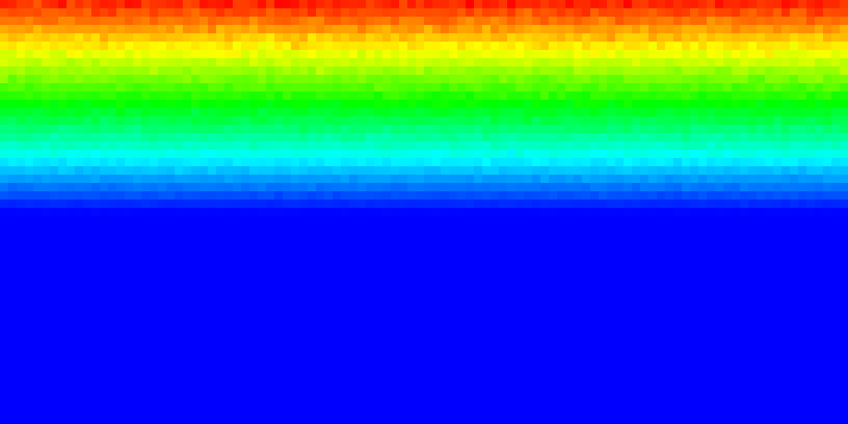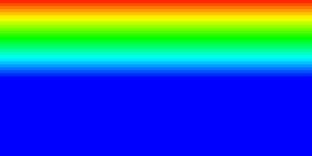I show you here also my implementation of the diffuse BSDF class:

class Diffuse : public BSDF {
public:
    explicit Diffuse(const Color3f& reflectance) : reflectance_(reflectance) {
        check_reflectance_value();
    }

    [[nodiscard]] Vector3f sample(/*const Vector3f& wo,*/ const de_vertexwahn::Point2f &sample_point) const override {
        Vector3f wi = square_to_cosine_hemisphere(sample_point);
        return wi;
    }

    [[nodiscard]] float pdf(const de_vertexwahn::Vector3f &wi) const override {
        if(cos_theta(wi) <= 0 || cos_theta(wi) <= 0) {
            return 0.f;
        }

        return pi_v<float> * cos_theta(wi);
    }

    [[nodiscard]] Color3f evaluate(const de_vertexwahn::Vector3f &wi, const de_vertexwahn::Vector3f &wo) const override {
        //if(wi.dot(wo) < 0)
        //    return Color3f{0.f};
        if(cos_theta(wo) <= 0 ||  cos_theta(wi) <= 0) {
            return Color3f{0.f};
        }

        return reflectance_ * (1.f / pi_v<float>);
    }

    const Color3f &reflectance() const {
        return reflectance_;
    }

private:
    void check_reflectance_value() const {
        for(int i = 0; i < 3; ++i) {
            if(reflectance_[i] < 0 || reflectance_[i] > 1) {
                throw std::runtime_error("Invalid reflectance value - must be in the range [0,1]");
            }
        }
    }

private:
    Color3f reflectance_;
};

Now we assume that you have implemented Diffuse BSDF class. How do we integrate it into our renderer? In my toy ray tracer, it looks like this:

Color trace(
        const Scene *scene,
        Sampler* sampler,
        Ray &ray,
        const int depth,
        Scalar *aovs = nullptr) const override {
    MediumEvent me;

    if (!scene->intersect(ray, me)) {
        return Color{0};
    }

    DCHECK(me.shape); // If there was a hit a valid shape is expected
    DCHECK(me.shape->bsdf()); // Every shape should have a BSDF

    // take care of emittance
    Color emitted_radiance{0};
    if(me.shape->is_emitter()) {
        emitted_radiance += me.shape->emitter()->evaluate();
    }

    // recursion limit
    if(depth >= max_depth_) return emitted_radiance;

    auto bsdf = me.shape->bsdf();
    auto sample_position = sampler->next_2d();
    Vector wo = me.sh_frame.to_local(-ray.direction);

    Vector wi = bsdf->sample(sample_position);
    assert(wi.norm() < Scalar{1.1} && wi.norm() > Scalar{.9});
    Scalar pdf = bsdf->pdf(wi);
    Color brdf_value = bsdf->evaluate(wi, wo);

    const Scalar EPSILON = Scalar{0.0001};
    Ray rn(me.p, me.sh_frame.to_world(wi), EPSILON, std::numeric_limits<Scalar>::infinity());
    Color indirect = trace(scene, sampler, rn, depth + 1);

    return emitted_radiance + indirect * brdf_value * cos_theta(wi) / pdf;
}

The code is similar to the pseudocode shown before. Additionally, you will find some conversion from world space to reflection space and back again.

In this section, we gained the following insights:

• A proper interface for a BSDF that supports diffuse materials can consist of sample, pdf, and evaluate functions
• The BSDF interface works only in a reflection coordinate system and is independent of the world space coordinate system

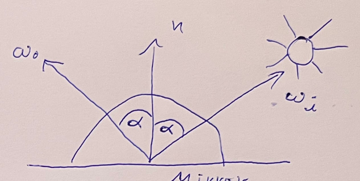
A Perfect Specular BSDF class #

In the following image you can see two spheres with a perfect specular reflection:

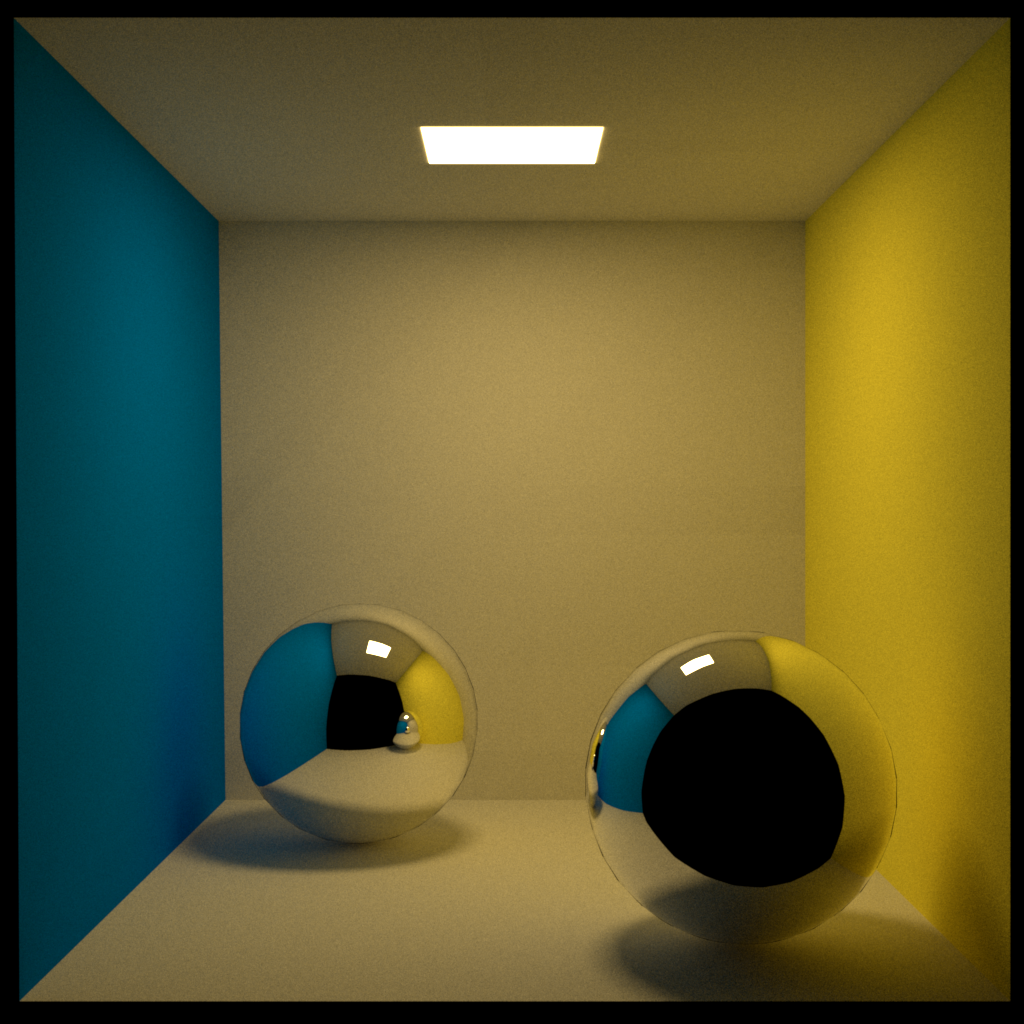
A perfect specular reflection (mirror reflection) has the property that light with some incident angle \(\alpha\) is reflected around the normal with exactly the same angle. The angle of incidence is equal to the angle of reflection:

The BRDF of a perfect mirror reflection looks like this, where \(\delta(x)\) denotes the Dirac Delta function:

Now lets consider how we can implement a BSDF class for perfect specular reflections (i.e. a perfect mirror material). Given the previously described interface, we will get into some problems:

• If we consider our BSDF interface again, we can see that the job of the sample method is to generate a sample \(\omega_i\) given two uniform random numbers within the domain \([0,1(\) . The probability that we hit exactly the mirror direction is almost 0. Therefore, a render that uses our BRDF interface will have a hard time rendering mirror reflections.
• The pdf will be always zero except if the sample is exactly in the mirror direction. In this case the probability will by \(\infty\) . This value will bring more problems when it comes to the division by this value in our trace function.

To work around those issues one option is to change BSDF interface. In the code for the diffuse BSDF interface, the `trace`` function looked like this:

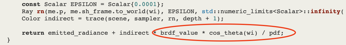
We now modify it this way:

Color value = bsdf->sample(bsdf_sample, sample_position);
...
Color indirect = trace(scene, sampler, rn, depth + 1);
return emitted_radiance + indirect * value;

The red ellipse is replaced by the magic variable value. The variable value is determined by the function sample. That means that the determination of the BRDF value, generating \(\omega_i\) , and computing the pdf is all done by the sample function now. So to say the sample function now generates only a multiplier for \(L_i\) .

So we change the sample method: We do not anymore return the sampled direction, but a multiplier for \(L_i\) , i.e. we change:

Vector3f sample(const Point2f& sample_point) const = 0;

to:

Color3f sample(const Point2f& sample_point) const = 0;

Same sample methods will need access to \(w_i\) or other things - to not get crazy about modifying always the interface we introduce a common struct BSDFSample that is handed over to each method in the BSDF interface:

strct BSDFSample {
    Vector3f wi;
    Vector3f wo;
}

class BSDF {
    [[nodiscard]] virtual Color3f sample(BSDFSample& sample, const Point2f& sample_point) const = 0;
    [[nodiscard]] virtual Scalar pdf(const BSDFSample& sample) const = 0;
    [[nodiscard]] virtual Color3f evaluate(const BSDFSample& sample) const = 0;
};

This new interface allows us to simplify the computation for perfect diffuse reflections as shown in Naive diffuse path tracing.

References #

• Rendering: Path Tracing I