Monte Carlo integration #
Uniform Monte Carlo estimator #
Assuming we are given an integral and want to determine its value \(F\) :
\(F = \int_{a}^{b} f(x) dx\)We now divide the right side by \(N\) and to compensate for this by summing up the integral \(N\) times:
\(F = \frac{1}{N} \sum_{i=0}^{N-1}{ \int_{a}^{b} f(x) dx }\)This looks first as a complete needless step but will bring us towards a nice result. We do a similar trick for the fraction \(\frac{1}{b-a}\) . We add this fraction as a multiplier inside the integral and compensate for this by multiplying the whole sum by \(b-a\) :
\(F = (b-a) \frac{1}{N} \sum_{i=0}^{N-1}{ \int_{a}^{b} f(x) \frac{1}{b-a} dx }\)Until now we only polluted a simple formula with some useless terms that can be totally eliminated when simplifying the equation again. Put when looking close at the changes we did - you can see that \(\frac{1}{b-a}\) is the probability density function ( \(p\) ) of a uniform distribution. Assuming the values for x are chosen uniform distributed between \(a\) and \(b\) we can write:
\(F = (b-a) \frac{1}{N} \sum_{i=0}^{N-1}{ \int_{a}^{b} f(x) p(x) dx }\)Where \(p(x)\) is the probability density function of a uniform distribution. Assuming that x is uniform distributed the integral is equal to the expected value \(\mu = \int_{a}^{b}{xf(x)dx}\) within the bounds of \(a\) and \(b\) . Therefore, the integral can be replaced with the expected value:
\(F = (b-a) \frac{1}{N} \sum_{i=0}^{N-1} E\left[f(X_i)\right]\)The expected value of a sum of random variables \(Y_i\) is the sum of their expected values:
\(E\left[\sum_{i=1}^{n} Y_i\right] = \sum_{i=1}^{n} E[Y_i]\)A constant \(c\) can be moved out of the expected value:
\(E[c Y ] = c E[Y]\)Applying this to our formula we get:
\(F = E\left[ (b-a) \frac{1}{N} \sum_{i=0}^{N-1} f(X_i)\right]\)The above equation gives the so called (uniform) Monte Carlo estimator and is denoted as \(\left\langle F^N \right\rangle\) :
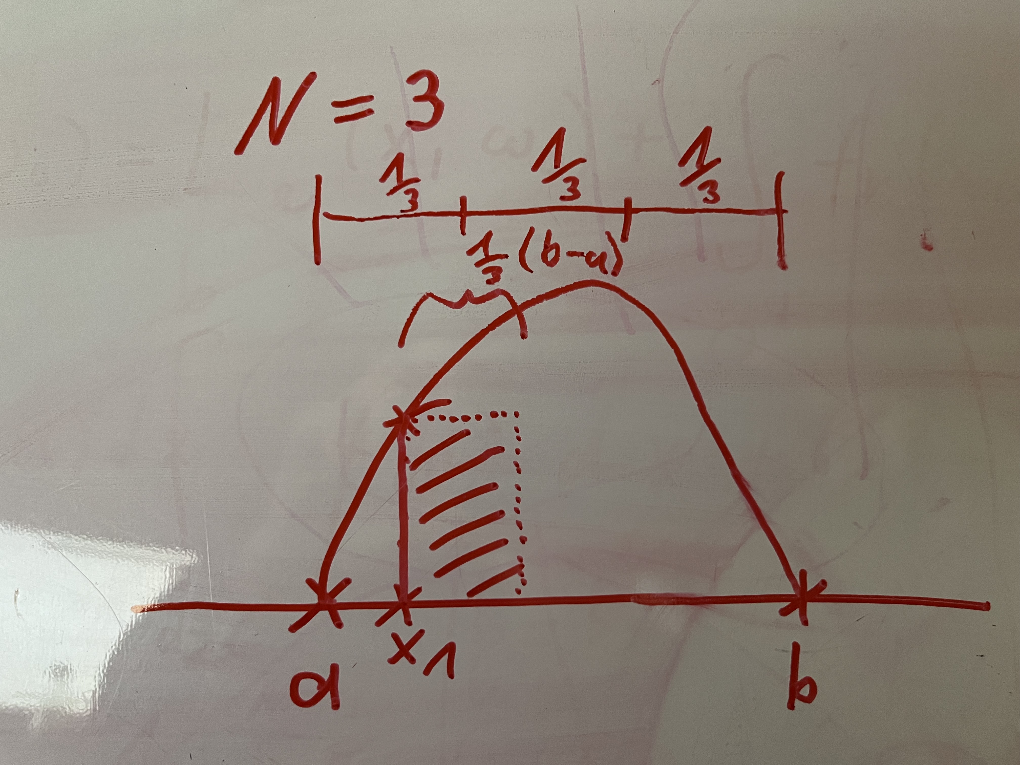
\(\left\langle F^N \right\rangle = (b-a) \frac{1}{N} \sum_{i=1}^{N} f(X_i)\)The \(N\) in the estimator defines how many samples are used to approximate the integral.
A geometrical interpretation of this (uniform) Monte Carlo estimator is that it is the area of a rectangle with width \((b-a) \frac{1}{N}\) and height \(f(X_i)\) . This is very similar to the rectangle rule.
Generalized Monte Carlo estimator #
The previous shown Monte Carlo estimator works when the chosen samples are uniformly distributed. Sometimes it can be very helpful if the samples do not need to be uniformly distributed, but can be chosen from any distribution function. The generalized Monte Carlo estimator is for that:
\(\left\langle F^N \right\rangle = \frac{1}{N} \sum_{i=0}^{N-1}{\frac{f(x_i)}{p(x_i)}}\) \(\int_a^b f(x) dx \approx \frac{1}{N} \sum_{i=0}^{N-1}{\frac{f(x_i)}{p(x_i)}}\)Importance Sampling #
Since the generalized Monte Carlo estimator gives us the freedom to choose an arbitrary PDF to sample your integral of interest, we can choose the PDF in a smart way that maybe helps us to approximate the integral of interest in a faster way than a simple uniform distribution.