Modified Phong BRDF #
Introduction #
Phong described in 1975 a lighting model that consist of a diffuse and a specular term [1]. Since the model does not have a physical basis Lafortune et al. proposed a modified version that is called the Modified Phong BRDF [2].
A reference image: Modified Phong BSDF in Mitsuba 0.5.0 #
A nice property that is shared by all physical based renderers is that they want to render the same physical correct image. To get a reference image for our expected result, we can pick a physical based renderer that supports the Modified Phong BRDF and create a reference image.
Mitsuba 0.5.0 supports the Modified Phong BRDF. Please note that newer versions of Mitsuba (e.g. 3.x) do not support the Modified Phong BRDF anymore, since this model is a bit outdated and replaced by more advanced models. Anyways, the Modified Phong BRDF is a good starting point to understand the basics of how to sample BRDFs.
In the Mitsuba 0.5.0 scene file a Modified Phong BRDF can be defined via:
<bsdf type="phong" id="modified_phong_brdf">
    <float name="exponent" value="30"/>
    <rgb name="diffuseReflectance" value="0.5"/>
    <rgb name="specularReflectance" value="0.2"/>
</bsdf>
When this material is applied to a sphere within a Cornell Box the output can look like this:
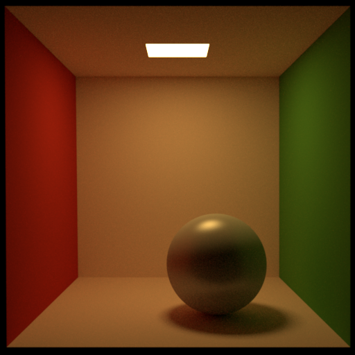
The whole scene description can be found here.
Bidirectional reflection distribution function (BRDF) #
The bidirectional reflection distribution function (BRDF) describes how a material reflects light. It is formally defined by [2]:
\(f_r(x, \omega_i, \omega_o) = \frac{dL_o(x_i,\omega_o)}{L_i(x, \omega_i)\cos{\theta_id\omega_i}}\)- \(x\) defines the position on the surface
- \(\omega_i\) (sometimes written as \(\Theta_i\) ) is the direction from which the light comes in defined in polar coordinates \((\varphi_i,\theta_i)\) , where \(\varphi_i\) and \(\theta_i\) describe the azimuth and evaluation angles. We do not need to define a radius value for this polar coordinate, since we are only interested in the direction.
- \(\omega_o\) (sometimes written as \(\Theta_o\) ) is the outgoing light direction defined in polar coordinates \((\varphi_o,\theta_o)\) , where \(\varphi_o\) and \(\theta_o\) describe the azimuth and evaluation angles. We do not need to define a radius value for this polar coordinate, since we are only interested in the direction.
- \(\cos{\theta_i}\) takes account of Lambert`s cosine law. The cosine between \(\omega_o\) and the surface normal at point \(x\)
- \(d\omega_i\) is a differential solid angle “around” \(\omega_i\)
- \(L_i(x,\omega_i)\) is the radiance incoming to point \(x\) along the direction \(\omega_i\) through \(d\omega_i\)
- \(dL_o(x,\omega_o)\) is the differential amount of reflected light towards \(\omega_o \)
There are materials that reflect light dependent on its wavelength \(\lambda\) . This wavelength dependency was ignored in the above definition. The above formula works only for a one specific wavelength and not a light spectrum. Let’s assume we consider only radiation with a single constant frequency from the visible spectrum, i. e. monochromatic light.
Helmholtz reciprocity #
According to the Helmholtz reciprocity the incoming and outgoing direction of light can be interchanged:
\(f_r(x, \omega_i, \omega_o) = f_r(x, \omega_o, \omega_i) \)// A physically based BRDF should obey the rule of reciprocity
void checkReciprocity(const Bxdf* bxdf) {
spinlock_mutex mutex;
ParrallRun<8,128>( [&]() {
const Vector wi = UniformSampleSphere(sort_rand_float(), sort_rand_float());
const Vector wo = UniformSampleSphere(sort_rand_float(), sort_rand_float());
const auto f0 = bxdf->F(wo, wi) * absCosTheta(wo);
const auto f1 = bxdf->F(wi, wo) * absCosTheta(wi);
std::lock_guard<spinlock_mutex> lock(mutex);
ASSERT_NEAR(f0.r, f1.r, 0.001f);
ASSERT_NEAR(f0.g, f1.g, 0.001f);
ASSERT_NEAR(f0.b, f1.b, 0.001f);
});
}
Definition #
The Modified Phong BRDF consist of an diffuse ( \(f_{r,d}\) ) and a specular ( \(f_{r,s}\) ) part:
\(f_r(x, \omega_i, \omega_o) = f_{r,d}(x, \omega_i, \omega_o) + f_{r,s}(x, \omega_i, \omega_o) = k_d \frac{1}{\pi} + k_s\frac{n+2}{2\pi}\cos^n\alpha\)where
- \(\alpha\) defines the angle between the perfect specular direction and the outgoing direction \(\omega_o\)
- \(k_d\) defines the reflection coefficient for the diffuse part of the BRDF
- \(k_s\) defines the reflection coefficient for the specular part of the BRDF
- \(n\) is a power exponent for the specular part. Higher values make the make specular reflection part sharper
To preserve energy conservation \(k_d + k_s \le 1\) must hold.
Implementation of a Modified Phong BRDF #
For a Modified Phong BRDF we need to implement the BSDF interface.
class ModifiedPhongBRDF : public BSDF {
    Color3f sample(BSDFSample& sample, const Point2f& sample_point);
    Scalar pdf(const BSDFSample& sample);
    Color3f evaluate(const BSDFSample& sample);
};
Evaluate #
Lets first focus on the implementation on the evaluate method.
How would a simple test look like?
Given
\(\omega_i = \omega_o = (0,0,1) \\ k_s = k_d = 0.5 \\ n = 10 \\\)Now lets compute \(f_r\) :
\(f_r(x,\omega_i,\omega_o) = k_d \frac{1}{\pi} + k_s\frac{n+2}{2\pi}\cos^n\alpha = \\ 0.5 \frac{1}{\pi} + 0.5 \frac{10+2}{2\pi} \cos^{10} 0 = \\ 0.5 \frac{1}{\pi} + 0.5 \frac{10+2}{2\pi} = \frac{7}{2\pi} \approx 1.11408\)A unit test for this can look like this:
TEST(Phong, evaluate) {
    PropertySet ps;
    ps.add_property("diffuseReflectance", Color3f{.5f});
    ps.add_property("specularReflectance", Color3f{.5f});
    ps.add_property("exponent", 10.f);

    Phong phong{ps};

    BSDFSample3f sample;
    sample.wo = Vector3f{0.f, 0.f, 1.f};
    sample.wi = Vector3f{0.f, 0.f, 1.f};

    Color3f result = phong.evaluate(sample);

    float abs_error = 0.001f;
    EXPECT_THAT(result.red(), testing::FloatNear( 7.f / (2.f * pi_v<float>), abs_error));
    EXPECT_THAT(result.green(), testing::FloatNear( 7.f / (2.f * pi_v<float>), abs_error));
    EXPECT_THAT(result.blue(), testing::FloatNear( 7.f / (2.f * pi_v<float>), abs_error));
}
No lets think about other test cases:
| \(\omega_i\) | \(\omega_o\) | \(k_s\) | \(k_d\) | n | \(f_r\) | Comment |
|---|---|---|---|---|---|---|
| (0,0,1) | (0,0,1) | 0.5 | 0.5 | 10 | \(\frac{7}{2\pi}\) | |
| (0,0,1) | (0,0,1) | 0.0 | 0.0 | 10 | 0 | No reflection |
| (0,0,1) | (0,0,1) | 0.0 | 1.0 | 10 | \(\frac{1}{\pi}\) | Only diffuse |
| (0,0,1) | (0,0,1) | 1.0 | 0.0 | 10 | \(\frac{6}{\pi}\) | Only specular |
PDF #
Calculus #
Speed is the derivation of time after location:
\(v(t) = \frac{dx}{dt}\)In the following diagram the “blue” line shows a 1D motion. Depending on the time \(t\) the position \(x\) changes:
TODO: FIX THIS GRAPH - note this is WIP and not correct

The red line shows the corresponding velocity for each point in time.
The average speed \(\bar{v}\) can be computed by
\(\bar{v} = \frac{\Delta x}{\Delta t} = \frac{x_2 - x_1}{t_2 - t_1}\)Partial differentiation #
References #
- https://computergraphics.stackexchange.com/questions/5502/phong-brdf-in-mitsuba-tungsten-and-agi
- https://www.youtube.com/@VrKomarov/videos
- https://www.youtube.com/watch?v=aolI_Rz0ZqY&t=1762s
- https://www.youtube.com/watch?v=XZ3w_jec1v8
- https://github.com/cs440-epfl
- https://github.com/voithos/muon/blob/main/muon/materials.cc
- https://github.com/ange-yaghi/manta-ray/blob/master/src/dielectric_media_interface.cpp
- https://github.com/JiayinCao/SORT/blob/master/src/unittests/bxdf.cpp
- https://www.open-std.org/JTC1/SC22/WG21/docs/papers/2023/p2996r1.html
- https://ashvardanian.com/posts/google-benchmark/
- https://www.youtube.com/watch?v=zduSFxRajkE Let’s build the GPT Tokenizer
- B. Phong,
Illumination for computer generated pictures,
Seminal graphics: pioneering efforts that shaped the field, 1975. [Online]. Available: https://api.semanticscholar.org/CorpusID:1439868 - E. Lafortune and Y. Willems, Using the modified Phong reflectance model for physically based rendering. Celestijnenlaan 200A, 3001 Heverlee, Belgium: Departement Computerwetenschappen, KU Leuven, 1994. [Online]. Available: https://www.cs.princeton.edu/courses/archive/fall03/cs526/papers/lafortune94.pdf